What Is Backpropagation? How AI 'Learns,' Explained via Error Backpropagation and Gradient Descent
When an AI 'learns,' what is it actually doing? We explain how a neural network adjusts its weights using three tools—the loss function, gradient descent (the descending-a-mountain analogy), and backpropagation—with diagrams, for non-specialists.
“AI learns.” “We train the model.” We see and hear phrases like these almost every day. But when an AI is learning, what is actually happening inside it? It’s not that a teacher is supplying answers, nor that the AI is reading a book and memorizing it. What actually happens is a relentlessly humble task: adjusting, just a tiny bit at a time, an enormous number of dials called “weights.”
The mechanism for doing that adjustment accurately and efficiently is the star of this article: backpropagation (error backpropagation) and gradient descent. These two are, so to speak, the “engine of learning” that powers nearly all of modern deep learning—from image recognition to large language models.
In the article What Is a Neural Network? we explained that an AI is made of a great many connected units (neurons). This article is its sequel. When we say a neural network “learns by adjusting its weights,” we dig into the “how” of that—splitting it into three tools, the loss function, gradient descent, and backpropagation—with math kept to a minimum.
Learning Means “Adjusting the Weights a Little at a Time”
A neural network takes an input (say, an image of a handwritten digit), computes through many units, and returns an output (an answer like “this is a 7”). Each connection between units has a number attached, called a weight. A weight is a dial that decides “how much to value this signal,” and in a large network there can be billions of them. This is the true identity of parameters.
A network that has just started learning has weights set to random initial values, so its answers are random too. Show it an image of “7” and it confidently gets it wrong: “this is a 2.” Learning is the task of using such mistakes as material to turn the weight dials, a little at a time, in the direction that approaches the correct answer. The problem is: how do you know which way, and how far, to turn billions of dials? Solving that is the job of the three tools we’ll look at next.
Tool 1: The Loss Function — Turning “How Wrong” Into a Single Number
To know which way to turn the dials, you first have to measure “how wrong are we right now.” That yardstick is the loss function. Loss bundles the “gap” between the answer the network produced and the true correct answer into a single number—0 if it’s perfectly correct, and larger the further off it is.
For example, if for an image of “7” the network answers “20% chance it’s a 7, 70% chance it’s a 2,” the gap from the correct answer is large and the loss is high. As learning progresses and it can answer “95% chance it’s a 7,” the loss becomes small. In other words, the goal of learning can be rephrased as finding the combination of weights that makes this loss as small as possible across all the training data. This converts the vague goal of “make it smart” into a problem mathematics can handle: “minimize a number called loss.”
Tool 2: Gradient Descent — Reducing Loss Like Descending a Foggy Mountain
Even saying “minimize the loss,” the combinations of billions of weights are astronomical, far too many to try all of them. This is where gradient descent comes in.
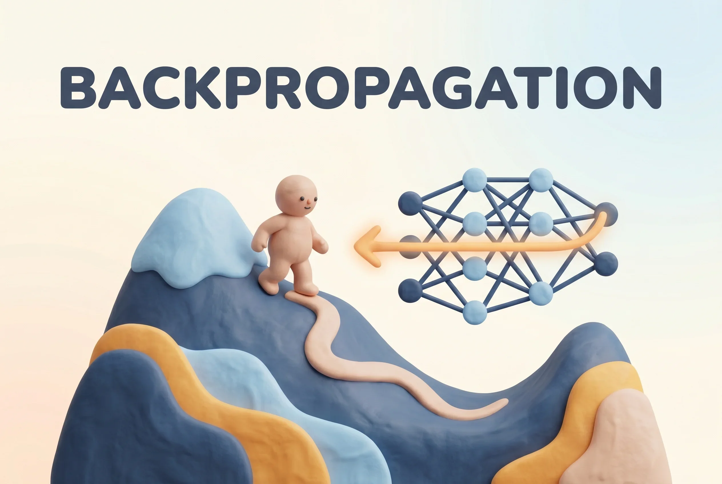
Wikipedia defines gradient descent as “a first-order iterative algorithm for minimizing a differentiable multivariate function”3. The mechanism is to advance, little by little, from a point in “the direction of the negative gradient of f at that point (−∇f)“3—that is, the direction of steepest descent. This is often explained with the analogy of descending a foggy mountain. Wikipedia likewise notes that a person on a mountain shrouded in thick fog, unable to see the whole, can only “look at the steepness of the hill at their current position, then proceed in the direction with the steepest descent”3.
Loss (height)
  \               ← you are here (current weight value)
    ●
     \  ↓ one step in the steep direction
       \●
         \   ↓ measure the slope again, step again
           \●____
                  \●___ ← valley floor (loss is minimal = goal of learning)
─────────────────────────► weight value
Measure the slope at your feet (the gradient), take a step in the steepest downhill direction. Where you land, measure the slope again, take another step. Repeat, and eventually you reach the valley floor (the weights at which loss is minimal)—this is the idea of gradient descent.
What decides the size of each step is a setting called the learning rate. Wikipedia points out that if the learning rate is “too small it would slow convergence, and too large it would lead to overshoot and divergence”3. If the stride is too small it takes forever to reach the valley floor; too large and you leap over the valley and ride up the opposite slope. Tuning this learning rate is one of the most fundamental and important adjustments in AI development.
| Learning rate | Analogy | Result |
|---|---|---|
| Too small | Tiptoeing in small steps | Takes far too long to reach the valley floor |
| Appropriate | Descending with a sensible stride | Approaches the valley floor efficiently |
| Too large | Bounding in giant leaps | Overshoots the valley—diverges, unstable |
Tool 3: Backpropagation — Assigning “Who Was How Much to Blame,” Working Backward
Gradient descent tells us “just go in the slope’s direction.” But a hard problem remains. For each of billions of weights, how do you efficiently compute “if I nudge it a little, how does the loss change” (i.e., the slope)? If you repeated “nudge this weight and measure the loss” one weight at a time, you’d never finish in any realistic amount of time.
Backpropagation (error backpropagation) elegantly solves this. In Wikipedia’s definition, it is a method that “efficiently computes the gradient of the loss with respect to the network weights for a single input–output example”2. The key is that it carries out that computation backward, one layer at a time, from the output side to the input side. In principle it “propagat[es] derivatives backward, one layer at a time, from the output layer to the input layer”2, and its true nature is an efficient application to neural networks of the chain rule (the derivative of composite functions) that even appears in high-school math2.
Intuitively, it helps to think of it this way. First, computation proceeds from input to output (the forward pass), and you find the gap between the answer produced and the correct answer—the error. Next, tracing that error backward from the output side to the input side, you apportion “how much each weight was responsible for the final mistake.”
[Forward pass] input → hidden layers → output → compute loss (error)
  ●──►●──►●──►●  "answered 2 for a 7. This much error."

[Backward pass] loss ← hidden layers ← output  apportion blame backward
  ●◄──●◄──●◄──●  compute at each layer "how much this weight drove the error"
        ↓
  adjust each weight "by its share of blame" via gradient descent
By analogy, it’s a retrospective on a failed team project. Working backward from the final failure (the output’s error), you trace from the back of the process to the front “how much each decision affected the result,” and work out each member’s (each weight’s) contribution (responsibility). What makes backpropagation excellent is that it can carry out this assignment of blame all at once, skipping wasteful computation. Wikipedia too explains that, compared with a naive approach, it gains efficiency by “not computing unnecessary intermediate values”2. Once the gradients of all weights are known, gradient descent then adjusts each weight by its share of blame—the repetition of forward pass, backward pass, and weight update is the learning of a neural network itself.
”Computing” and “Updating” Are Separate Jobs
Here’s a distinction that’s easy to confuse. Backpropagation and gradient descent are often lumped together, but their roles differ. Wikipedia cautions that “strictly speaking, the term backpropagation refers only to an algorithm for efficiently computing the gradient, not how the gradient is used”2.
In other words, backpropagation is the part that “computes the slope (gradient) of each weight,” and gradient descent is the part that “uses that gradient to update the weights.” The former works out on the map “which way is downhill,” and the latter actually takes a step in that direction. Dividing the labor, the two together make up the single act of learning.
Practical Tricks: Mini-Batches and Epochs
In theory, it’s most accurate to compute loss over “all the training data.” But doing this every time on datasets of millions or billions of examples means enormous computation for a single step. So in practice, stochastic gradient descent (SGD) is used.
In Wikipedia’s definition, SGD “replaces the actual gradient (calculated from the entire data set) by an estimate thereof (calculated from a randomly selected subset of the data)“4. Instead of looking at everything to choose an accurate step, it looks at only part of the data, makes a rough guess “downhill is roughly this way,” and quickly takes a step. Wikipedia describes this as a trade-off of “faster iterations in exchange for a lower convergence rate”4.
In reality, it’s common to process data not one example at a time but in small groups of tens to hundreds, called mini-batches4. And going through the training data once is called an epoch. In learning, you repeat this epoch many times while shuffling the data, polishing the weights until the loss becomes small enough (converges). A phrase like “trained for 3 epochs” means the dials were adjusted using three passes’ worth of the training data.
| Term | Meaning |
|---|---|
| Batch (all data) | Compute the gradient over all training data (accurate but heavy) |
| Mini-batch | Compute the gradient over groups of tens to hundreds (the practical standard)4 |
| Epoch | Going through the training data once |
| Learning rate | The step size. Too small is slow; too large diverges3 |
Why This Mechanism Is “the Foundation of AI”
Backpropagation is by no means a new idea. What made it widely known was the 1986 paper “Learning representations by back-propagating errors”1, published in the academic journal Nature by David Rumelhart, Geoffrey Hinton, and Ronald Williams. The original states that the procedure “repeatedly adjusts the weights of the connections in the network so as to minimize a measure of the difference between the actual output vector of the net and the desired output vector”1—exactly the explanation we’ve seen in this article.
What made this paper a landmark was another observation. As you adjust the weights, “internal ‘hidden’ units which are not part of the input or output come to represent important features of the task domain”1. Without humans teaching it “this is an eye, this is a contour,” the network acquires meaningful features on its own through learning—this “automatic acquisition of representations” became the core of later deep learning. Wikipedia, too, credits this 1986 work as having “became highly cited, contributed to the popularization of backpropagation, and coincided with the resurging research interest in neural networks during the 1980s”2. (Incidentally, the co-author Geoffrey Hinton listed here is one of the researchers later called, together with Yoshua Bengio and Yann LeCun, the “Godfathers of AI.”)
Today’s giant models like GPT and Claude, and AIs that recognize images too, at the root of their learning repeat—an unimaginable number of times—the cycle we’ve seen in this article: measure the loss, find the gradient via backpropagation, and update the weights a little at a time. Behind the flashy capabilities, what keeps quietly turning is an accumulation of humble computation, like descending a foggy mountain one step at a time.
If you’d like to learn more about how learning works, read the foundational What Is a Neural Network?; for failures that happen when learning works too well, read What Is Overfitting?; and for how to fit a trained model to a purpose afterward, read What Is Fine-Tuning?. Together they bring the substance of the phrase “AI learns” into sharper relief.
Sources
- Learning representations by back-propagating errors - David Rumelhart, Geoffrey Hinton, Ronald Williams, Nature vol. 323, pp. 533–536, 1986. The original paper that popularized backpropagation
- Backpropagation - Wikipedia (definition of backpropagation; chain rule; distinction between computing the gradient and using it; history)
- Gradient descent - Wikipedia (definition of gradient descent; negative gradient; learning rate; the foggy-mountain analogy)
- Stochastic gradient descent - Wikipedia (SGD; mini-batches)
Was this article helpful?
Thank you!
Received. Thank you!