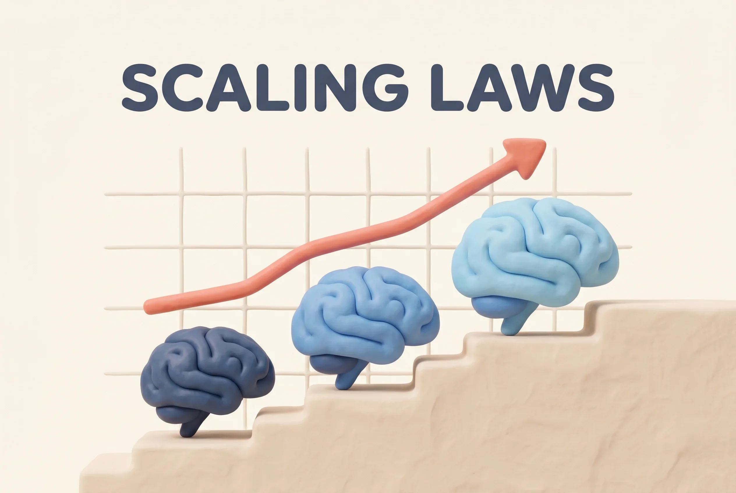
What Are Scaling Laws? Why AI Gets Smarter When You Make It Bigger, and the Emergent Abilities Debate
Why does AI get smarter as you add more parameters, data, and compute? We explain scaling laws—where loss falls along a power law—covering the Kaplan (2020) vs. Chinchilla (2022) clash and the debate over emergent abilities, with diagrams for non-specialists.
For the past several years, the AI industry has been gripped by a peculiar fever. Companies raced to pour resources into more parameters, more data, and more GPUs: GPT-3’s 175 billion parameters, computing infrastructure investments worth hundreds of billions of yen, the constant refrain that “the next model will be even bigger.” Behind it all was not mere chest-thumping but a single empirical rule: scaling laws.
Put simply, scaling laws are the discovery that “the larger the model, the more training data, and the more compute you use, the more an AI’s performance improves—in a predictable, smooth way.” And that improvement is so regular that it forms a straight line when plotted. The “predictable” part was decisive. If you can roughly calculate, before running the experiment, “how much more I need to invest to get how much smarter,” then a massive investment becomes not a gamble but an investment decision.
In this article, we dig into why AI gets smarter when you make it bigger, using scaling laws as a guide. We tackle—head-on, but with almost no math—the paper by Kaplan et al. (2020)1 that started it all, the 2022 Chinchilla paper2 that overturned its conclusion by pointing out “you don’t have enough data,” and the debate over emergent abilities34—the idea that beyond a certain scale, an AI suddenly acquires new capabilities. Knowing what parameters and tokens mean makes this easier to read, but the article is written so you can follow it without that background.
What Are Scaling Laws? An Empirical Rule That “Predicts” Performance
To borrow Wikipedia’s definition, a scaling law is “an empirical scaling law that describes how neural network performance changes as key factors are scaled up or down”5. The “key factors” here can be roughly organized into three:
- Model size (N): the number of parameters—the AI’s “brain size.”
- Data size (D): the number of tokens used for training—the “amount of teaching material” the AI reads.
- Compute (C): the total amount of computation spent on training—the “effort invested,” proportional to GPUs × time.
And the “performance” being measured is, in most cases, a number called loss. Loss represents “how far off the AI’s predictions are”—the smaller, the smarter. What scaling laws claim is that this loss falls along a power law with respect to each of N, D, and C.
“Power law” sounds unfamiliar, but the idea is simple. It’s a relationship where “multiplying one side by 10 makes the other drop by a fixed proportion,” and on a graph with both axes in log scale it becomes a clean straight line. Kaplan et al.’s original paper reported that this relationship holds across “more than seven orders of magnitude”1. Multiplying by ten, seven times over—in other words, across a range of ten million-fold, the same straight line kept extending.
Loss L (log scale)
 high │\
      │  \____  "The more model, data, and compute,
      │      \\   the more loss falls (along a power law)"
      │         \\
      │            \\____
 low  │                \\____
      └────────────────────────────► Compute C (log scale)
       small                       large
This “linearity” is the heart of scaling laws. If it’s a straight line, you can extrapolate—predict—the performance of a giant model you haven’t built yet, like laying a ruler down and extending the line. “You won’t know until you try” became “you can estimate by calculating”—and that profoundly changed R&D decision-making.
”Scale” Matters More Than “Shape”
Another important point in Kaplan et al.’s findings was that the fine shape of the network barely matters. The original paper states that “other architectural details such as network width or depth have minimal effects within a wide range”1.
This is counterintuitive. Normally you’d expect the skill of the design—“how to stack the layers,” “how to connect them”—to determine performance. Yet in the world of scaling laws, making things bigger works far better than tweaking the design. This insight resonated with what AI researcher Richard Sutton later called “The Bitter Lesson”—that general methods able to leverage computation ultimately win out over methods crafted with human ingenuity—and it created the era’s prevailing mood of “just scale it up.”
Kaplan 2020: The Starting Gun for Going Big
Scaling laws were systematically demonstrated in the 2020 paper “Scaling Laws for Neural Language Models”1 by ten authors including Jared Kaplan, Sam McCandlish, and Dario Amodei (many of whom later founded Anthropic). They systematically measured the loss of language models against model size, data size, and compute, and discovered the power law described above.
The paper’s most influential claim concerned sample efficiency. In the original’s words: “Larger models are significantly more sample-efficient, such that optimally compute-efficient training involves training very large models on a relatively modest amount of data and stopping significantly before convergence”1.
Broken down, it means this: given the same compute budget, you’re better off training a large model partway than training a small model until it’s fully exhausted its data. In Kaplan et al.’s analysis, when you increase the compute budget, the optimal move is to direct most of it toward enlarging the model. Wikipedia summarizes this as “N_opt(C) ∝ C^0.73, D_opt(C) ∝ C^0.27”5: put most of any added compute (exponent 0.73) into model size, and only a little (exponent 0.27) into data.
This conclusion sent a clear message to the industry: “When in doubt, make the model bigger first.” The race for hundreds-of-billions-of-parameters models that followed GPT-3 (175 billion parameters) was carried out along this prescription.
Chinchilla 2022: “You Don’t Have Enough Data”
But in 2022, a paper by Jordan Hoffmann et al. at DeepMind, “Training Compute-Optimal Large Language Models”2, threw cold water on this trend. It is commonly known as the Chinchilla paper.
Their question was simple: “Given a compute budget, what is the optimal combination of model size and number of training tokens?”2. After training more than 400 models ranging from 70 million to over 16 billion parameters, experimenting on 5 billion to 500 billion tokens, they reached a startling conclusion. In the original’s words: “current large language models are significantly undertrained”2.
In other words, the giant models of the day had grown their parameters while their data failed to keep up—they were buried treasure. Chinchilla’s prescription was clear: “for compute-optimal training, the model size and the number of training tokens should be scaled equally: for every doubling of model size the number of training tokens should also be doubled”2. This stands in direct opposition to Kaplan’s “model-heavy” approach (in Wikipedia’s framing, Hoffmann et al. give “N_opt(C) ∝ C^0.5, D_opt(C) ∝ C^0.5”5—growing model and data equally).
And they proved the theory with a single model.
| Gopher (old style) | Chinchilla (compute-optimal) | |
|---|---|---|
| Parameters | 280B | 70B (one-quarter) |
| Training data | less | 4× |
| Compute budget | same | same |
| MMLU benchmark | — | 67.5% average (>7% over Gopher)2 |
Chinchilla is a model that, with the same compute budget as its stablemate Gopher (280 billion parameters), cut its parameters to one-quarter—70 billion—and used 4× the data instead2. As a result, in the original’s words, “Chinchilla uniformly and significantly outperforms Gopher (280B), GPT-3 (175B), Jurassic-1 (178B), and Megatron-Turing NLG (530B) on a large range of downstream evaluation tasks”2. With a smaller body, it beat models 4 to 7 times its size. On MMLU—one of the AI benchmarks—it scored 67.5% on average, surpassing Gopher by over 7%2.
There was another benefit not to be overlooked. Being smaller, it “uses substantially less compute for fine-tuning and inference, greatly facilitating downstream usage”2. It wasn’t just smarter—it was cheaper to use.
From this finding, a practical rule of thumb of “about 20 tokens per parameter” (D ≈ 20N) became widely known5. The intuition is that a 70-billion-parameter model is compute-optimal when trained on roughly 1.4 trillion tokens. After Chinchilla, the industry’s conventional wisdom quietly shifted from an era of “blindly increasing parameters” to one of “balancing against data.” The “exhaustion of high-quality training data” so often discussed today traces back, at its root, to this teaching of Chinchilla’s.
 How to allocate the same compute budget?

 Kaplan 2020          Chinchilla 2022
 ┌─────────────┐      ┌─────────────┐
 │ Model  ████ │      │ Model  ██   │
 │ Data   █    │      │ Data   ██   │
 └─────────────┘      └─────────────┘
 "Model-heavy"        "Model and data equally"
Emergent Abilities: Powers That Appear “Suddenly” Beyond a Scale
Scaling laws were, so to speak, a story of a continuous, predictable world where “loss falls smoothly.” But in 2022, a paper by Jason Wei et al., “Emergent Abilities of Large Language Models”3, reported a discontinuous phenomenon lurking beneath that smoothness: emergent abilities.
Wei et al.’s definition is clear: “We consider an ability to be emergent if it is not present in smaller models but is present in larger models. Thus, emergent abilities cannot be predicted simply by extrapolating the performance of smaller models”3. The paper opens by noting that scaling is known to improve performance “predictably,” then declares: “this paper instead discusses an unpredictable phenomenon”3.
Concretely, on tasks like three-digit addition or complex reasoning, the model couldn’t solve them at all while small (an accuracy no better than random guessing), then suddenly became able to solve them the moment it crossed a certain parameter scale. The performance graph, having crawled along the ground for a long time, leaps upward from a single point as if scaling a cliff. Techniques like chain-of-thought (CoT)—“making the model show its work makes it smarter”—were reported to have this same emergent character: the effect appears only in models that have reached a certain scale.
This finding surprised people in two ways. One was sharpness—a capability switching from “absent” to “present” almost instantaneously. The other was unpredictability—you can’t tell in advance at what scale it will happen4. If that’s truly the case, then “the next giant model may suddenly acquire abilities we never anticipated.” This was both a source of hope for AI’s potential and a source of concern over safety.
”It’s a Mirage”: The Counterargument
But science scrutinizes the most exciting claims the hardest. In 2023, Rylan Schaeffer et al., in a provocatively titled paper “Are Emergent Abilities of Large Language Models a Mirage?”4, questioned the very phenomenon of emergence.
Their argument runs like this. Emergent abilities appear “due to the researcher’s choice of metric rather than due to fundamental changes in model behavior with scale”4. More concretely: “nonlinear or discontinuous metrics produce apparent emergent abilities, whereas linear or continuous metrics produce smooth, continuous predictable changes in model performance”4.
For example, if you use a strict scoring scheme—“one point only if you get it completely right, zero if even a single character is off” (a discontinuous metric)—then even if the model is improving little by little, its score stays at zero for a long time and then suddenly jumps to one. But if you measure “how close to correct” continuously, you find that improvement had been progressing smoothly all along, behind the scenes. In other words, the “cliff” wasn’t a cliff of capability but a cliff of the ruler.
This debate didn’t end with either side fully winning; rather, it brought a fundamental question to the surface: how should we measure and talk about AI capabilities? What matters is the stance of distinguishing, when you hear that “AI suddenly got smarter,” whether it’s truly a leap in capability or an effect of how it was measured. Before getting swept up in flashy benchmark numbers, ask what was measured and how. The lesson Mirage left behind applies to us as news readers too.
| Emergence camp (Wei 2022)3 | Mirage camp (Schaeffer 2023)4 | |
|---|---|---|
| How abilities appear | Suddenly emerge at a certain scale | Actually change smoothly and continuously |
| The “cliff” in the graph | A qualitative leap in capability | An artifact of a discontinuous metric |
| Predictability | Cannot be predicted by extrapolation | Predictable with a continuous metric |
What Scaling Laws Teach Us
To sum up, the story of scaling laws has unfolded in three stages. First, we learned that performance improves predictably along a power law with scale (Kaplan 2020). Second, its optimal allocation was corrected from “model-heavy” to “balanced against data” (Chinchilla 2022). Third, it is being asked whether, beneath the smooth improvement, there is a leap that can be called “emergence,” or whether that is a product of how we measure (Wei vs. Schaeffer).
This story offers several practical perspectives even for readers not directly involved with AI.
One is seeing why massive AI investment was “calculation” rather than “gambling.” Scaling laws predict, to some degree, the return on the resources invested. That’s exactly why companies could confidently pour hundreds of billions of yen into computing infrastructure. Conversely, when those predictions start to break down—when high-quality data runs out, say, or the straight line of the power law begins to flatten—that becomes a sign that the industry’s premises are shaking.
Another is the lesson Chinchilla showed: size alone is not value. Parameter counts tend to become marketing slogans, but what really works is the balance with data, and a small, smart, cheap model is easier to use in practice. This is a still-living idea, one that connects to the later rise of mixture-of-experts (MoE) and compact high-performance models, and to the thinking behind reasoning models that “adjust intelligence at inference time” as well.
And finally, as Mirage urges, the numbers used to describe AI capabilities always come with a caveat of “how it was measured.” Scaling laws are a powerful compass, but not the map itself. Increase the scale and many measures of performance will rise—but reading what that rise means is, in the end, still a human’s job.
If you’d like to learn more about how AI “learns,” read What Is a Neural Network?; for another technique alongside scale—“making it think along the way”—read What Is a Reasoning Model?. Together, they bring the “story of scale” seen here into three dimensions.
Sources
- Scaling Laws for Neural Language Models - Jared Kaplan et al., 2020. The original scaling-laws paper (power-law loss and sample efficiency)
- Training Compute-Optimal Large Language Models - Jordan Hoffmann et al. (DeepMind), 2022. The Chinchilla paper (compute-optimal balance of model and data)
- Emergent Abilities of Large Language Models - Jason Wei et al., 2022. Definition and report of emergent abilities
- Are Emergent Abilities of Large Language Models a Mirage? - Rylan Schaeffer et al., 2023. Counterargument to emergent abilities (metric-choice explanation)
- Neural scaling law - Wikipedia (definition of scaling laws; N/D/C/L; the Kaplan–Hoffmann allocation difference; 20 tokens per parameter)
Was this article helpful?
Thank you!
Received. Thank you!