What Is a Neural Network? How AI 'Learns,' Explained from the Ground Up
What is a neural network? From its building blocks—neurons, weights, activation functions, and layers—to how it learns through backpropagation and gradient descent, plus the history of the perceptron's limits and revival. A clear, illustrated guide to the foundation of generative AI.
ChatGPT writes essays, image generators paint pictures, and self-driving cars pick out pedestrians. These technologies look completely different, yet they share one common foundation: the neural network. Even the large language models (LLMs) at the heart of the generative AI boom are, on the inside, nothing but enormous neural networks.
The cloud giant AWS defines a neural network as “a method in artificial intelligence (AI) that teaches computers to process data in a way that is inspired by the human brain”2. Put differently, once you understand how a neural network works, you can see the root of why today’s AI can “learn” at all—and why it sometimes gets things wrong.
This article digs into what a neural network is from three angles—its building blocks, how it learns, and its history—using almost no mathematics. It is the explanation of the “engine” sitting one level deeper than our overview of the difference between AI, machine learning, and deep learning.
Why “Inspired by the Brain”?
Our brains contain countless cells called neurons. AWS explains that “human brain cells, called neurons, form a complex, highly interconnected network and send electrical signals to each other to help humans process information”2. Each individual neuron is simple—an element that “receives signals from other cells and fires a signal to the next cell once a certain strength is exceeded.” Yet when tens of billions of them connect, complex functions like language, vision, and memory emerge.
A neural network mimics this idea—“connect many simple elements and complex behavior emerges”—with mathematics and computers. The crucial caveat is that this is only an inspiration, not a precise copy of the brain. Artificial neurons are far more simplified than biological ones. Even so, this simplified model became a surprisingly powerful mechanism that drives real-world AI.
Building Blocks: Nodes, Weights, Activation Functions, and Layers
A neural network is made of four kinds of parts. Let’s look at them in turn.
Nodes (Neurons) and Weights
The smallest unit of the network is the node (artificial neuron). A single node takes multiple inputs and combines them into one output number. The strength of the connection between inputs is represented by a weight. AWS explains that “a number, called weight, represents the connections between one node and another. The weight is a positive number if one node excites another, or negative if one node suppresses the other”2.
A weight is, in effect, a knob that sets how easily a signal passes between nodes. Inputs with large weights strongly affect the output; small (or negative) ones have weak influence. As we will see, for a neural network to “learn” is nothing more than adjusting these countless weights little by little.
Activation Functions
A node doesn’t stop at multiplying inputs by weights and summing them. It passes that sum through a transformation called an activation function before producing its output. Wikipedia defines it as “a function that calculates the output of the node based on its individual inputs and their weights”5. Much as a biological neuron “fires once a certain strength is exceeded,” the activation function decides how the summed input is converted into an output.
What matters decisively here is that the activation function is non-linear (a curved transformation). Wikipedia notes that “nontrivial problems can be solved using only a few nodes if the activation function is nonlinear”5, whereas if everything is linear, “the entire network is equivalent to a single-layer model”5. In other words, no matter how many layers you stack, depth means nothing if the activation function is linear. Common activation functions include the smooth S-shaped sigmoid and ReLU (max(0, x)), which zeroes out negative inputs and passes positive ones through unchanged5. ReLU was widely used in the 2012 image-recognition model AlexNet and others, and became a driving force in making the training of deep networks practical5.
Layers
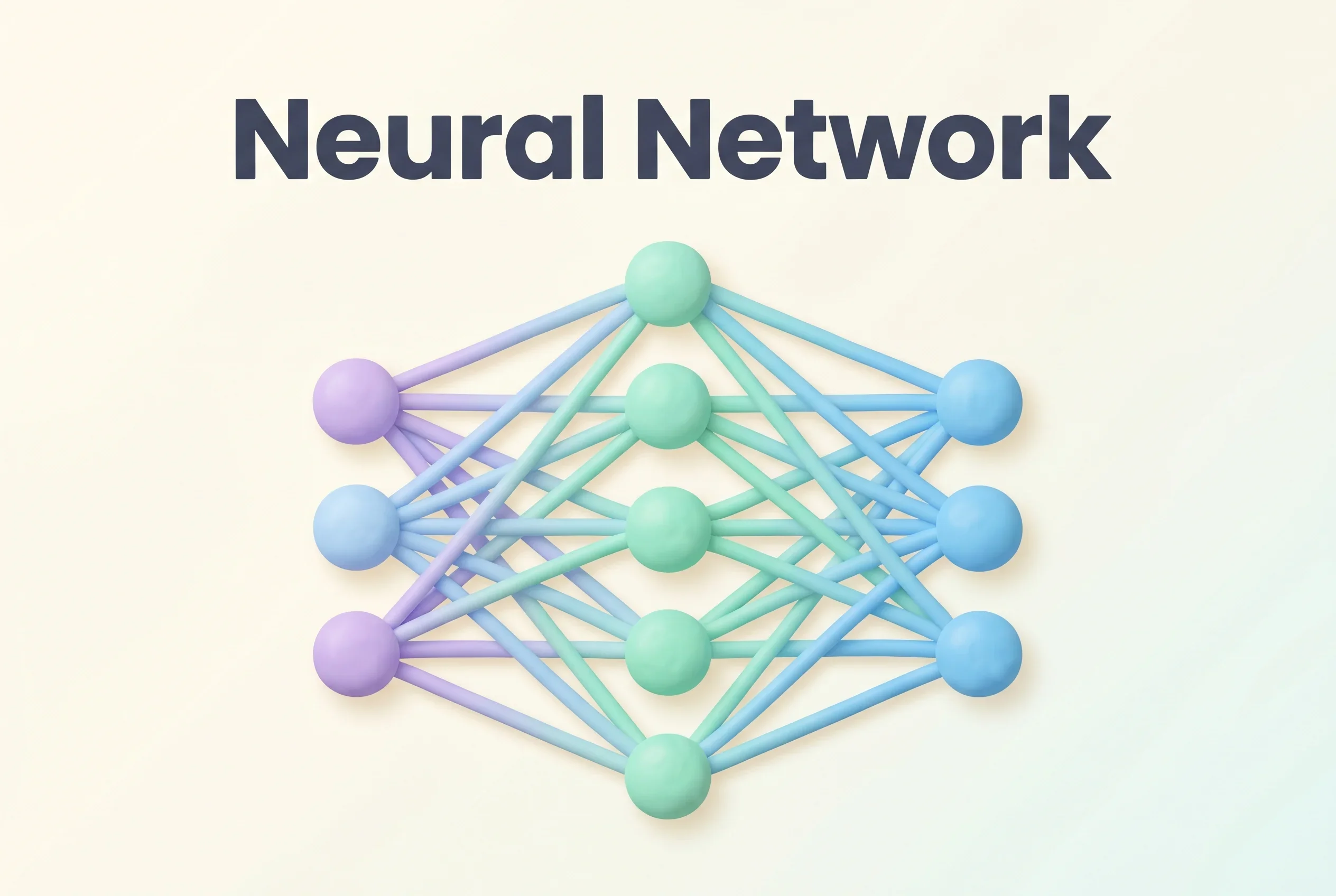
Nodes are organized into units called layers, and stacking layers builds the network. There are three kinds of layers with different roles.
| Layer type | Role | AWS description2 |
|---|---|---|
| Input layer | The entrance that receives data from outside | ”Information from the outside world enters the artificial neural network from the input layer. Input nodes process the data, analyze or categorize it, and pass it on to the next layer.” |
| Hidden layer | Intermediate processing that transforms information step by step | ”Each hidden layer analyzes the output from the previous layer, processes it further, and passes it on to the next layer.” Networks can have many of them. |
| Output layer | The exit that produces the final answer | ”The output layer gives the final result of all the data processing by the artificial neural network.” |
Data enters at the input layer, is transformed as it passes through the hidden layers one at a time, and emerges as an answer at the output layer. This “calculation in which a signal flows one way, from entrance to exit,” is called forward propagation. Feed in an image of a handwritten digit, for example: the input layer receives the brightness of each pixel, the hidden layers capture features like “lines” and “curves,” and the output layer returns the answer “this is a 7.”
How Does It “Learn”? Backpropagation and Gradient Descent
So far we’ve covered how a finished network produces an answer. But how does the crucial part—learning, that is, finding the right weights—actually happen? This is the heart of a neural network, and it can be explained in three steps.
Step 1: Check the answer (compute the loss). A freshly initialized network has random weights and produces answers riddled with errors. So we measure the size of the gap between the network’s answer and the “true correct answer” as a single number called the loss. A larger loss means “more badly wrong.” The goal of learning is to find the combination of weights that makes this loss as small as possible.
Step 2: Find which way to adjust (compute the gradient). For each of the countless weights, we need to know whether increasing or decreasing it will reduce the loss. The “direction that reduces the loss fastest,” expressed mathematically, is the gradient. This is where backpropagation shines. Wikipedia defines backpropagation as “a gradient computation method commonly used for training a neural network in computing parameter updates”4, and describes its work as efficiently computing “the gradient of the loss with respect to the network weights for a single input–output example”4. As the name implies, it traces the error produced at the output layer backward toward the input layer, assigning to each weight how much it contributed to the error.
Step 3: Adjust just a little (gradient descent). Once the gradient is known, the weights are nudged ever so slightly in the direction that reduces the loss. Wikipedia describes this as “changing model parameters in the negative direction of the gradient, such as by stochastic gradient descent”4. Because it resembles descending a mountain in fog by taking one step at a time in the steepest downhill direction at your feet, it is called gradient descent.
Repeating these three steps millions or billions of times over vast amounts of data, the loss gradually drops and the weights converge toward values that “produce correct answers.” This is the true nature of how a neural network learns.
| Step | What it does | Keyword |
|---|---|---|
| 1 | Measure the gap between answer and truth | Loss |
| 2 | Find the direction to fix each weight | Gradient / backpropagation |
| 3 | Nudge weights in the loss-reducing direction | Gradient descent |
What’s striking is that this mechanism works without humans having to teach it the features. In the 1986 founding paper, David Rumelhart, Geoffrey Hinton, and Ronald Williams reported that repeatedly adjusting weights via backpropagation causes the internal hidden units to “represent important features of the task domain”1. Without a programmer defining “this is what a 7 looks like,” the network discovers “seven-ness” on its own from many examples.
History: The Perceptron’s Setback and Revival
Neural networks did not develop in a straight line. There was a drama of hope, disillusionment, and revival.
The starting point was the perceptron, published by psychologist Frank Rosenblatt in a 1958 paper3. The “Mark I Perceptron,” first publicly demonstrated on June 23, 1960, was a machine that read images using 400 photocells arranged in a 20×20 grid3. The idea that “a machine learns from experience” drew enormous attention.
But the early (single-layer) perceptron had a fundamental limitation. Wikipedia explains that “single-layer perceptrons are only capable of learning linearly separable patterns”3. In 1969, the book Perceptrons by Marvin Minsky and Seymour Papert showed that this class of network could not even learn the simple logical function XOR (exclusive or)3. This point—though it could in fact be solved by going multi-layer—was widely received as “neural networks have inherent limits,” and is said to have ushered in an “AI winter” of dwindling research funding3.
What ended the winter was precisely the backpropagation we saw above. Wikipedia notes that the 1986 Nature paper by Rumelhart, Hinton, and Williams “contributed to the popularization of backpropagation, and coincided with the resurging research interest in neural networks during the 1980s”4. Problems unsolvable with one layer became solvable through the combination of multi-layer networks with hidden layers and backpropagation, which could train them efficiently.
| Year | Event | Significance |
|---|---|---|
| 1958 | Rosenblatt publishes the perceptron3 | The prototype of a “learning machine” |
| 1969 | Minsky & Papert, Perceptrons3 | Points out single-layer limits (XOR); the winter begins |
| 1986 | The backpropagation paper (Rumelhart et al.)14 | Multi-layer training becomes practical; interest revives |
| 2010s onward | The rise of deep learning6 | Data and GPUs let multi-layer networks flourish |
Why Go “Deep”? Learning Features Hierarchically
Modern AI uses deep networks with many stacked hidden layers—that is, deep learning. Wikipedia defines deep learning as “utilizing multilayered neural networks to perform tasks such as classification, regression, and representation learning”6, and explains that the adjective “deep” refers to “the use of multiple layers (ranging from three to several hundred or thousands) in the network”—more precisely, “the number of layers through which the data is transformed”6.
Why does going deeper make a network smarter? The key is hierarchical representation learning. Wikipedia states that “a hierarchy of layers is used to transform input data into a progressively more abstract and composite representation”6. Take face recognition: shallow layers capture “edges” (boundaries of light and dark), middle layers capture parts like “eyes” and “noses,” and deep layers capture “the whole face”—the level of abstraction rises as you climb the layers. And the decisive difference from older methods is that “features are not hand-crafted and the model discovers useful feature representations from the data automatically”6.
There is theoretical backing, too. Networks with non-linear activation functions are interpreted via the “universal approximation theorem,” and Wikipedia notes that even a two-layer network “can be proven to be a universal function approximator”5. Given enough size, a neural network can in principle approximate any input-to-output relationship, however complex—a powerful property that is the source of the versatility to “handle images, audio, and language with the same mechanism.”
The Link to Modern AI: It All Sits on Top of Neural Networks
Today’s flagship AI systems can be organized as applications of neural networks. The Transformer that handles text, the LLMs built on it, the diffusion models that generate images—each is internally a network of stacked layers, and the principle of learning is the same repetition we saw here: “measure the loss, find the gradient by backpropagation, fix the weights by gradient descent.”
The “7B” or “70B” in a model’s name—its parameter count—is exactly the number of weights that appeared again and again in this article. The more parameters, the more complex the relationships the network can represent, but the more computation its training and operation require. And adjusting a pretrained network’s weights further for a specific purpose is fine-tuning, while tuning it to match human preferences is RLHF. Both stand on the great principle of “adjusting the weights.”
Limits: Powerful but Not Omnipotent
Finally, a word on the limits. A neural network is powerful only when there is plenty of data and computation; if the training data is biased, it learns that bias along with everything else. Its “black box” nature—the difficulty of explaining what happened inside to reach a conclusion—also poses challenges in fields like medicine and finance where accountability is demanded. Even hallucination—confidently outputting plausible errors—stems at its root from this very mechanism: the network merely learned to minimize the loss against correct answers, without understanding truth itself.
Even so, it is undeniable that the humble idea of “connecting many simple nodes, propagating errors backward, and fixing weights little by little” became the foundation of today’s AI revolution after half a century of ups and downs. If you want to learn more about what is stacked on top of neural networks, reading on into the Transformer, the core of language AI, or the parameter count that expresses a model’s size, will bring the meaning of the phrase “AI learns” into three-dimensional focus.
Sources
- Learning representations by back-propagating errors - Rumelhart, Hinton & Williams, Nature 323:533-536 (1986). The original paper on backpropagation
- What is a Neural Network? - Amazon Web Services (AWS) explainer on neural networks
- Perceptron - Wikipedia (history of the perceptron and the XOR problem)
- Backpropagation - Wikipedia (definition and history of backpropagation)
- Activation function - Wikipedia (activation functions and universal approximation)
- Deep learning - Wikipedia (deep learning and representation learning)
Was this article helpful?
Thank you!
Received. Thank you!